Intro to CNNs
Convolutional Neural Networks are a special type of Deep Neural Networks, used almost exclusively for solving problems in the field of computer vision.
They are a state-of-the-art technique, proven to be much more effective than any other Machine Learning algorithm for image processing tasks.
Basic architecture
- A generic architecture of a CNN uses two main types of layers:
- Convolutional Layer
- MaxPooling Layer
- Although earlier architectures used Fully Connected Layers in the end, modern architectures don’t use them anymore.
This is how a CNN can be visualised:
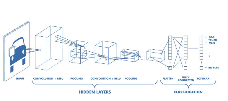
Looks complicated? Let’s break it down!
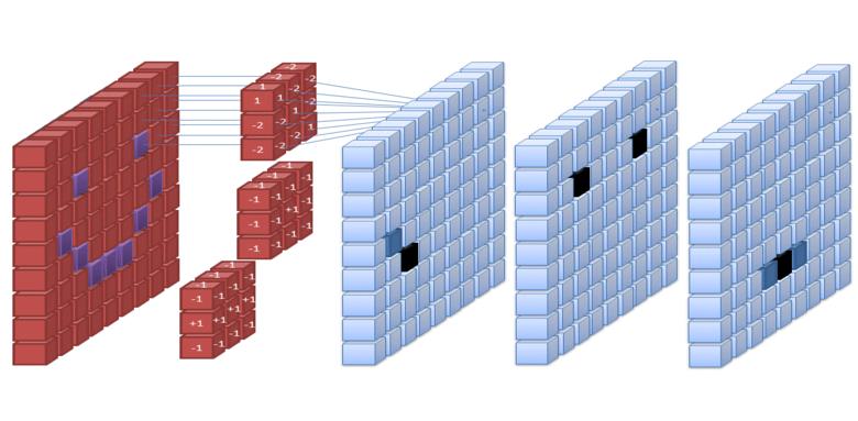
What is a convolution?
In deep learning, the term refers to the matrix correlation operation, where one of the matrices is the input image or an intermediate layer; the other matrix is called a kernel.
The gif below should give you a basic idea of what a 4 pix * 3 pix convolution looks like:
The number of steps taken sideways or down after every matrix multiplication is known as stride. In the above case, stride = 1.
Now let’s take a look at MaxPool
The gif below shows a 6 pix * 3 pix maxpooling operation with stride = 3.
In MaxPool, for a M * M matrix (say A) pooled with size N * N, take a N * N chunk from A and pick out the largest value from that chunk. Simple, right?
Introducing Keras
Keras is a Deep Learning library, now integrated with Google’s popular DL framework, Tensorflow.
We shall use this library to make a simple CNN.
So what do we do now?
One thing about the Deep Learning community - people are rather fond of pets. So let’s make a CNN that classifies whether a given image is that of a dog or a cat!
Time to get our hands dirty!
The code below assumes you are working on Google Colab, on a GPU instance. Feel free to set up Tensorflow GPU on your local machine.
Why GPU? Because it speeds up training by several times ( > 100x easy).
# install dependencies
!pip install keras
Next, let’s write a function to assemble the model. In Keras, this process is almost like putting together a jigsaw puzzle - all the pieces are given to you, and you need to figure out how they fit.
from keras import Sequential
from keras.layers import *

def create_model():

    # A sequential model is one where all layers come one after the other. This is good enough for simple models.
    model = Sequential()

    # model.add(...) appends a new layer to our model

    # The input layer. The shape is of the form (height, width, channels). Here, channels=3 because we are using  RGB images.
    model.add(InputLayer(input_shape=(150, 150, 3)))

    # Next, we perform a convolution operation with a 3*3 matrix. This is the matrix that the model "learns". Stride = 1 by default
    # Input shape to this layer: (150, 150, 3)
    # Output shape from this layer: (148, 148, 32)
    model.add(Conv2D(filters=32, kernel_size=(3, 3)))

    # Mathematically, BatchNormalization() makes the variance of incoming data 0.
    # Practically, it reduces the iterations required by the model to learn the next convolution matrix.
    model.add(BatchNormalization())

    # Finally, add the activation function.
    model.add(LeakyReLU(alpha=0.1))

    # Next, add a MaxPool layer.
    # This selects the most prominent feature from the pooled chunk.
    # Input shape to this layer: (148, 148, 32)
    # Output shape from this layer: (74, 74, 32). As you can see, height and width have been halved.
    # This reduces the amount of processing required in the following layers by a factor of 4, albeit at a cost of some features.
    # This is the reason we pick the largest value, to allow the most prominent features to move forward, discarding all others.
    # By default, this usees a 2 * 2 pool with stride = 2.
    model.add(MaxPooling2D())


    # Some more layers
    model.add(Conv2D(filters=64, kernel_size=(3, 3)))
    model.add(BatchNormalization())
    model.add(LeakyReLU(alpha=0.1))

    model.add(MaxPooling2D())

    model.add(Conv2D(filters=128, kernel_size=(3, 3)))
    model.add(BatchNormalization())
    model.add(LeakyReLU(alpha=0.1))

    model.add(Conv2D(filters=256, kernel_size=(3, 3)))
    model.add(BatchNormalization())
    model.add(LeakyReLU(alpha=0.1))

    model.add(MaxPooling2D())


    # Now here we have something interesting - A Conv2D layer with kernel size 1 * 1.
    # The purpose of this is to reduce the number of channels from the previous layer.
    # Think of it like this: MaxPool reduces X and Y dimensions; 1 * 1 Convolution reduces the Z dimension.
    model.add(Conv2D(filters=16, kernel_size=(1, 1), activation="relu"))


    # Continue adding layers:

    model.add(Conv2D(filters=32, kernel_size=(3, 3)))
    model.add(BatchNormalization())
    model.add(LeakyReLU(alpha=0.1))

    model.add(Conv2D(filters=64, kernel_size=(3, 3)))
    model.add(BatchNormalization())
    model.add(LeakyReLU(alpha=0.1))

    model.add(Conv2D(filters=128, kernel_size=(3, 3)))
    model.add(BatchNormalization())
    model.add(LeakyReLU(alpha=0.1))

    model.add(MaxPooling2D())
    model.add(Conv2D(filters=32, kernel_size=(1, 1), activation="relu"))

    model.add(Conv2D(filters=64, kernel_size=(3, 3)))
    model.add(BatchNormalization())
    model.add(LeakyReLU(alpha=0.1))

    model.add(Conv2D(filters=256, kernel_size=(3, 3)))

    # Finally, we add the layer that gives the output of the network.
    model.add(Conv2D(filters=1, kernel_size=(1, 1), use_bias=False))

    # This reduces a multidimentional array to a single dimensional array.
    # The purpose of this is to simply reshape the array output from the previous layer to the shape we require: A single number
    model.add(Flatten())

    # The following layer maps the single number in the range [0, 1] telling us whether the image is a cat or a dog.
    model.add(Activation("sigmoid"))

    # Now, we 'compile' the model. The optimizer and loss mentioned below are beyond the scope of this blog; I'll address them in future posts.
    # Do search for them yourself though.
    # "metrics" here is the set of values displayed during training. For now, we are only concerned with how accurately our model classifies cats and dogs.
    model.compile(optimizer="adam", loss="binary_crossentropy", metrics=["accuracy"])
    return model
Why have we built the model the way we have? Let’s find out!
cnn = create_model()
cnn.summary()
See some pattern?
The model has been constructed in such a way that the 150 * 150 * 3 input image is reduced to a 1 * 1 * 1 output. This output is then reshaped.
Even though you may not have the luxury of reducing every image input of every model to this ideal shape, the current implementation is good enough to get started.
Now that we have the model, let’s get the data to train the model on.
!wget https://download.microsoft.com/download/3/E/1/3E1C3F21-ECDB-4869-8368-6DEBA77B919F/kagglecatsanddogs_3367a.zip
!unzip -q kagglecatsanddogs_3367a.zip
The images will be in folders “PetImages/Cat” and “PetImages/Dog”.
There are 25000 images total, 12,500 images for each class. Additionally, there is a “Thumbs.db” file in each folder, which we do not need.
Let’s create a training and testing set from them.
First, create folders “train” and “test”, each having subfolders “Cat” and “Dog”
!mkdir train
!mkdir train/Cat
!mkdir train/Dog

!mkdir test
!mkdir test/Cat
!mkdir test/Dog
Next, create the datasets:
import os

CAT_IMG_PATH = "PetImages/Cat"
DOG_IMG_PATH = "PetImages/Dog"

CAT_IMG_DIR = os.listdir(CAT_IMG_PATH)
DOG_IMG_DIR = os.listdir(DOG_IMG_PATH)

CAT_TRAIN_PATH = "train/Cat"
CAT_TEST_PATH = "test/Cat"
DOG_TRAIN_PATH = "train/Dog"
DOG_TEST_PATH = "test/Dog"


# Use 10000 images of each class as training images, and 2500 images as testing images.

for i in range(10000):
    os.rename (
        CAT_IMG_PATH + "/" + CAT_IMG_DIR[i],
        CAT_TRAIN_PATH + "/" + CAT_IMG_DIR[i]
    )
    os.rename (
        DOG_IMG_PATH + "/" + DOG_IMG_DIR[i],
        DOG_TRAIN_PATH + "/" + DOG_IMG_DIR[i]
    )

for i in range(10000, 12501):
    os.rename (
        CAT_IMG_PATH + "/" + CAT_IMG_DIR[i],
        CAT_TEST_PATH + "/" + CAT_IMG_DIR[i]
    )
    os.rename (
        DOG_IMG_PATH + "/" + DOG_IMG_DIR[i],
        DOG_TEST_PATH + "/" + DOG_IMG_DIR[i]
    )
We now have our datasets ready. But, we need some way to feed this data into the model. Again, Keras comes to the rescue.
Keras has a built-in module called preprocessing, with a submodule called image. We shall use this to feed data into the network.
Look at the function below:
from keras.preprocessing.image import *

def get_data_loader():
    data_generator = ImageDataGenerator()
    data_flow = data_generator.flow_from_directory(
                    directory="train",
                    target_size=(150, 150),
                    classes=['Dog', 'Cat'],
                    batch_size=32,
                    class_mode="binary"
                )

    return data_flow
Some details about the above function:
ImageDataGenerator is a class in the image module. It’s use is self-explainatory.
flow_from_directory is a method of this class, that feeds data into the network, one batch at a time.
The name of the folder containing the training classes is given as a parameter to the function.
Each subfolder represents a class, and contains images of that class.
A batch is a small subset of the dataset fed into the network. Training takes place after one batch has been completely processed.
The term class_mode depends on the neural network architecture. Observe the last layer of the network. It is a single output unit, followed by Sigmoid activation.
General rule of thumb:
- Single output + Sigmoid -> class_mode=”binary”
- Multiple outputs + Softmax -> class_mode=”categorical”
It is highly recommended that you search for the terms you don’t understand on the internet, and/or your PU math textbooks.
Finally, the time has come! Let’s train the model we have created to the dataset we have worked so hard to assemble!
data_loader = get_data_loader()

# epoch: One training iteration is called an epoch.
# steps_per_epoch: No. of batches in one training iteration to be processed.
cnn.fit_generator(data_loader, steps_per_epoch=128, epochs=10)
You may get some errors saying that some image cannot be loaded, or such. This may happen if the particular image is corrupt.
In such cases, simply delete the image file with the following line:
!rm path/to/image
This will not have any major impact on training, since the number of images used is very large.
The following files were corrupt when I ran the code:
train/Cat/666.jpg
train/Dog/11702.jpg
The output after every epoch should contain a loss and an acc value.
If you have implemented the CNN correctly, the loss should gradually decrease, while acc should gradually increase.
Well, that’s it! You have successfully trained your network!
Let’s try it out on an image from the testing set.
import numpy as np
TEST_IMG = "test/<Cat or Dog>/<Any image file>"

# load_img and img_to_array are functions in keras.preprocessing.image
img = load_img(TEST_IMG, target_size=(150, 150))
img = img_to_array(img)

# This is required since keras takes input in batches.
img = np.expand_dims(img, axis=0)

result = cnn.predict(img)
print(result)
You should get a single decimal value as output. If the value > 0.5, the image is predicted to be of a cat. Otherwise, it is predicted to be of a dog.
Let’s check the accuracy of the model on the entire testing set.
correct = 0

CAT_TEST_DIR = os.listdir(CAT_TEST_PATH)
DOG_TEST_DIR = os.listdir(DOG_TEST_PATH)

for i in range(2500):
    img = load_img(CAT_TEST_PATH + "/" + CAT_TEST_DIR[i], target_size=(150, 150))
    img = img_to_array(img)

    img = np.expand_dims(img, axis=0)

    result = cnn.predict(img)

    # Converts [[value]] to value
    result = np.squeeze(result)

    if result > 0.5:
        # Image is correctly classified as cat
        correct += 1

for i in range(2500):
    img = load_img(DOG_TEST_PATH + "/" + DOG_TEST_DIR[i], target_size=(150, 150))
    img = img_to_array(img)

    img = np.expand_dims(img, axis=0)

    result = cnn.predict(img)

    # Converts [[value]] to value
    result = np.squeeze(result)

    if result < 0.5:
        # Image is correctly classified as dog
        correct += 1

print(correct*100.0 / 5000)
The output of the above code gives the percentage of images classified correctly.